Line Rasterization#

../_images/zigle_line.png — Drawing lines at 5° intervals#

This used Alois Zigl's error algorithm

When inspecting the Bresenham algorithm it was apparent that the position of the next pixel is computed using the displacement differences between the actual and theoretical lines. Depending on how steep the gradient is, the algorithm is biased to select pixels either above or below the theoretical line.

../_images/show_zigl_line.png — Line drawn from (x0, y0) to (x1, y1) showing the pixels activated for the rasterization algorithm.#

The line is drawn down the page as on a monitor.

The green, blue and dark grey pixels are activated by this algorithm which are the same that would be activated by the Bresenham algorithm.

Alois Zigl has a slightly different approach to Bresenham.

Starting from an implicit line equation

\[\begin{split}(x_1 - x_0) \, (y - y_0) - (x - x_0) \, (y_1 - y_0) & = 0 \\ \Delta{x} & = x_1 - x_0 \\ \Delta{y} & = y_1 - y_0\end{split}\]

As we move along the line we can say that the error ε, the difference between the pixel centre and theoretical line, is

\[ε = (y - y_0) \, \Delta{x} - (x - x_0) \, \Delta{y}\]

Note

Look carefully at the signs of the expressions. When computing the error in the x-direction we use the negative Δy, and for the y-direction use the positive Δx.

Building on the example from Alois Zigl a straight line starts and finishes from (1, 1) to (6, 5), it has difference values of Δx=5 and Δy=4, as we move one pixel away from the start, a shift in the x-direction has a smaller error than a shift in the y-direction, in fact the after swopping the differences, Δx and Δy, they become the errors, with a sign change in the x-direction.

Moving diagonally the error is

\[ε_{xy} = (y + 1 - y_0) \, \Delta{x} - (x + 1 - x_0) \, \Delta{y} = ε + \Delta{x} - \Delta{y}\]

Moving in the x and y directions

\[\begin{split}ε_x & = (y + 1 - y_0) \, \Delta{x} - (x - x_0) \, \Delta{y} = ε_{xy} + \Delta{y} \\ ε_y & = (y - y_0) \, \Delta{x} - (x + 1 - x_0) \, \Delta{y} = ε_{xy} - \Delta{x}\end{split}\]

The first step's error becomes

\[ε_1 = (y_0 + 1 - y_0) \, \Delta{x} - (x_0 + 1 - x_0) \, \Delta{y} = \Delta{x} - \Delta{y}\]

Moving from (x0, y0) to the centre of (x1, y1), the start pixel has by definition no error (green). The diagonal pixel(blue) e1 is (x+1, y+1) giving an error of 5 (0 + 5) in the y-direction (+dx) and -4 (0 - 4) in the x-direction, resulting in +1 (5 - 4). At the blue pixel there is a choice of the grey pixels (x+1, y+2), (x+2, y+1) or (x+2, y+2). The first pixel has an error of ex=6 (1 + 5), the second has an error ey=-3 (1 - 4) and the third an error of exy=2 (1 + 1). The darker grey pixel is chosen because it only has an error of +2. The next diagonal (x+3, y+3) has an error of +3, but is not chosen because the pixel (x+3, y+2) only has an error of -2. Starting from this pixel (x+3, y+2) the diagonal at (x+4, y+3) has an error of -1 (-2 +1). Although the Zigl's method is different, the result is exactly the same as for Bresenham's algorithm.

This concept is very powerful and Alois has extended it to plotting ellipses, circles and Bezier curves, all of which can then be antialiased.

../_images/eight_fold_zigl.png — Corrected Zigl Algorithm drawing in all sectors, x and y coordinates and differences flipped.#

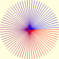
The line with a differences of 10 and 3 is telling, if the algorithm shows the pattern correctly then it should be universal. Check the line pattern against an algorithm that is known to be correct .

The following is a python script based on Alois' C program

Show/Hide Zigl Algorithm Basic Line

def plotLine(draw, pta, ptb, fill='black', width=1):
 x0, y0 = pta
 x1, y1 = ptb
 dx = abs(x1 - x0)
 dy = -abs(y1 - y0)
 sx = 1 if x0 < x1 else -1
 sy = 1 if y0 < y1 else -1
 err = dx + dy                # error value e_xy

 for x in range (x0, x1+1):
     draw.point([x0, y0], fill= fill)
     e2 = err<<1
     if e2 >= dy:             # e_xy + e_x > 0
         err += dy
         x0 += sx
     if e2 <= dx:             # e_xy + e_y < 0
         err += dx
         y0 += sy

As it stands this script only works on a gentle incline, when the slope is steep the line is foreshortened. However all is not lost! Use the method developed later for the antialiased line, it almost works in all octants except for vertical lines. Change the range conditions to account for steep conditions, this then enables vertical lines to show.

Show/Hide Zigl Algorithm Universal Line

def plotLine(draw, pta, ptb, fill='black', width=1):
 x0, y0 = pta
 x1, y1 = ptb

 dx = x1 - x0 # abs
 dy = y1 - y0 # -abs

 sx = 1 if dx > 0 else -1
 sy = 1 if dy > 0 else -1

 dx = abs(dx)
 dy = abs(dy)

 err = dx - dy # +
 dr = dx + 1 if dx > dy else dy + 1 # better plotting when steep

 for x in range (dr): #  x0, x1+1
     draw.point([x0, y0], fill= fill)
     e2 = err<<1
     if e2 >= -dx: # dy
         err -= dy # += dy
         x0 += sx
     if e2 <= dy: # dx
         err += dx
         y0 += sy

There are similarities with the second Bresenham algorithm when making it universal. Changes were also made to the Alois' definition of sx and sy (x- and y-sign), so that the comparison was made with zero.

BUT

Warning

The lines are not totally accurate. The antialiased lines plot the right points with the right colour, but the main line does not follow the Bresenham line exactly, the antialiasing fills in the points left out by the main line and the main line fills in those left out by the antialiasing. The final result is correct, but when trying to make antialiased arrows by switching off one side or other of antialiasing there are unwanted light antialiasing pixels left behind that in fact had been plotted by the main plot.

When the line is steep swop the main differences/errors.

Show/Hide Zigl Algorithm Corrected Line with flipped coordinates

def plotLine(draw, pta, ptb, fill='black', width=1):
x0, y0 = pta
x1, y1 = ptb

dx = dx0 = abs(x1 - x0)
dy = dy0 = abs(y1 - y0)
sx = 1 if x0 < x1 else -1
sy = 1 if y0 < y1 else -1

if dx0 > dy0:       # gentle incline
    dy = -dy
    dr = dx0 + 1
else:               # steep slope
    dx = -dx
    dr = dy0 + 1
    dx, dy = dy, dx
err = dx + dy

for j in range (dr):
    draw.point([x0, y0], fill= fill)
    e2 = err<<1
    if e2 >= dy:
        err += dy
        if dx0 > dy0:
            x0 += sx
        else:
            y0 += sy
    if e2 <= dx:
        err += dx
        if dx0 > dy0:
            y0 += sy
        else:
            x0 += sx

Test this out on a line that changes 10 in the x-coordinate and 3 in the y-coordinate, now make it plot in all 8 sectors.

Show/Hide Testing Algorithms draw in all 8 sectors

if __name__ == "__main__":
    w,h = 41,41

    image = Image.new('RGB', (w,h), '#FFFFDD')
    drawl = ImageDraw.Draw(image)

    a = (26,23),(23,26),(17,26),(14,23),(14,17),(17,14),(23,14),(26,17)
    b = (36,26),(26,36),(14,36),(4,26) ,(4,14), (14,4), (26,4) ,(36,14)

    for i in range(len(a)):
        plotLine(drawl, [a[i][0], a[i][1]], [b[i][0], b[i][1]],
            fill='black')

    image.show()

After running this script check it against a Bresenham and standard Pil line in particular note the patterns of long and short lines, these should match no matter which algorithm is used.

Line Rasterization#

This Page