Circles#
Mid-Point Algorithm#
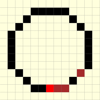
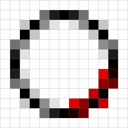
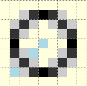
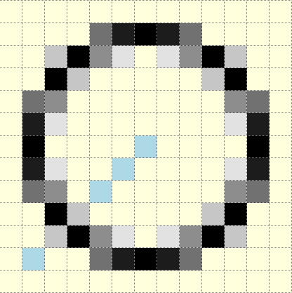
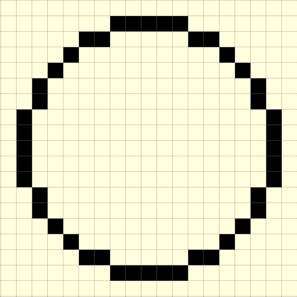
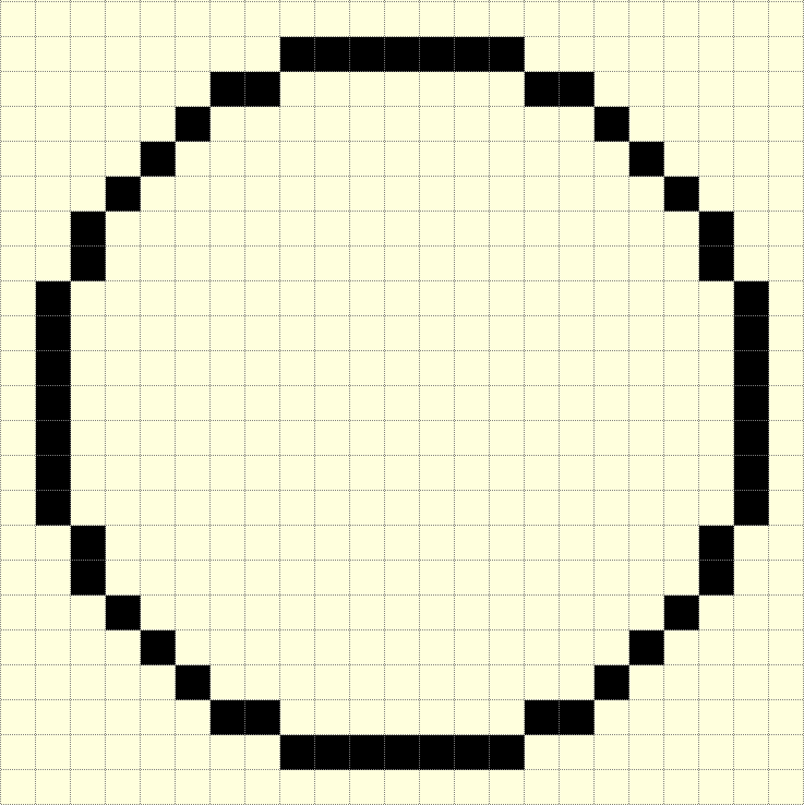
Circle radius 5 using mid point algorithm#
Start at the bottom (red), then progress by increasing x and sometimes decrease y. There is some duplication of points, shown by the black between two brown pixels. This is rectified later.
The main reason for looking at Bresenham and other derivatives is for the antialiased circle, from which we can derive the antialiased arc. When drawing plain circles use the PIL ellipse and arc methods whilst for thick circles use concentric circles and thick arcs use pieslices.

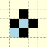
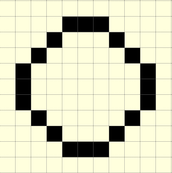
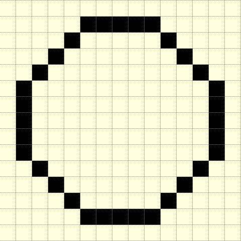
Eight way symmetry used in drawing circle.#
Not all scripts use the starting point (x=0, y=-r) shown by the blue sector. The advantage of this sector is that both x and y increase with a positive step change, the other sector where both x and y increase with a positive step change is almost opposite (4th sector).
The Bresenham circle and its derivative, the mid-point algorithm, operate in a similar fashion to the line algorithm. Since the circle is symmetrical it can be divided into octants of a circle, so these algorithms have 8 places where the pixel is plotted, but only one set of pixels are tested, the others are copies. Even though the algorithm assumes the circle centre is at the origin (0, 0) it can easily be transposed to the actual circle centre. The circle in the script below is calculated in the second octant:
def plotpoints(dr, xm, ym, x,y, fill):
   dr.point([xm+x, ym+y], 'brown')
   dr.point([ym+y, xm+x], fill)
   dr.point([ym+y, xm-x], fill)
   dr.point([xm+x, ym-y], fill)
   dr.point([xm-x, ym-y], fill)
   dr.point([xm-y, ym-x], fill)
   dr.point([xm-x, ym+y], fill)
   dr.point([xm-y, ym+x], fill)

def plotCircle(dr, xm, ym, r):
   # draw a black aliased circle on a light background

   x = 0
   y = r               # IV. quadrant from bottom top to right
   dr.point ([xm, ym+r], 'red')
   dr.point ([xm, ym-r], 'black')
   dr.point ([xm-r, ym], 'black')
   dr.point ([xm+r, ym], 'black')
   e = 5/4 - r

   while x < y:
     if e < 0:
         e = e + 2*x + 3
     else:
         e = e + 2*(x-y) + 5
         y -= 1
     x += 1
     plotpoints(dr, xm, ym, x,y, (0,0,0))
The variable e is used to determine whether the difference, or error, at the
mid point is positive or not and move only in the x-direction or move in the
negative y-direction. As it steps the error is updated by an amount computed
for the respective direction.
There are 2 good references on the mid-point algorithm, Computer Graphics Principles and Practice in C by James D. Foley Andries van Dam Steven K. Feiner John F. Hughes or try Bresenham's Circle Drawing Algorithm. When making thick circles it was found useful to combine part of the mid-point algorithm with the following algorithm by Alois Zigl.
Alois Zigl Algorithms#
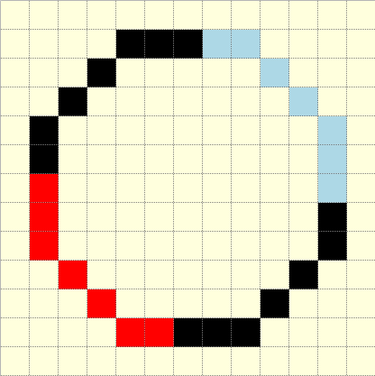
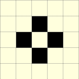
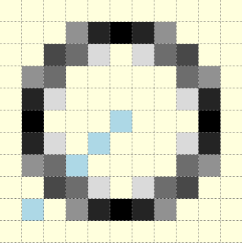
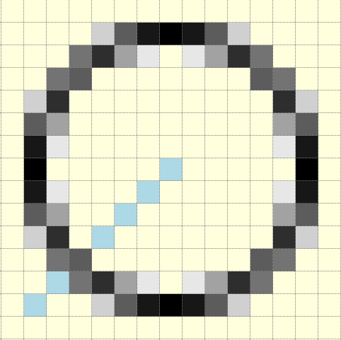
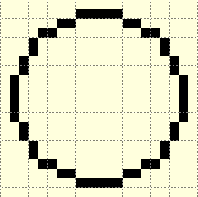
Circle radius 5 using Zigl's algorithm#
The algorithm starts at the left, and plots a circle quadrant (in red) which is copied to the other three quadrants.
The algorithm used by Alois Zigl only requires 4 common pixel plotting commands. The computation has both x and y-values increasing, the y-values slightly more than the x-values. When displaying the 2nd quadrant note that the x-values are negative (this will become positive when adding the centre x-value for plotting).
Just as with the line, the differences (errors) found in this algorithm can be used to generate the colour for antialiasing pixels.

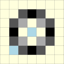
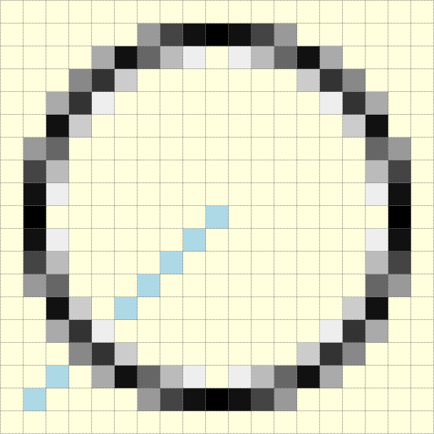
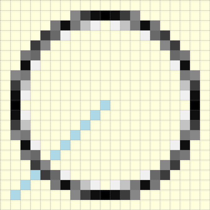
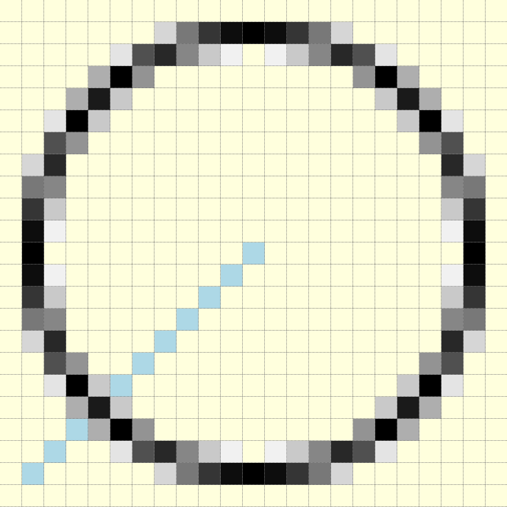
The differences (errors) in one quadrant for a circle with radius of 5#
Note how the differences increase from the centre outwards. The light grey squares are a scaled 5 pixel rasterized circle. A scaled circle of 5 pixels is drawn in blue.
The difference values in the other 3 sectors will be mirrored.
Moving outwards the differences change at a faster rate, so the centre (difference -25) on a 5 pixel circle is 3 pixel diagonals away from the circumference, between (-3,3) and (-4,4), whereas a further 2 pixels outwards (-5,5) there is a difference of 25. Using the differences as they stand would favour antialiasing on the inside.
Circumference Pixels
start (-5,0)
mid (-4,3)
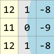
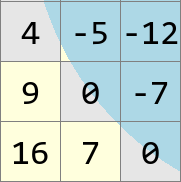
Look what happens around a pixel that sits exactly on the circumference. The starting pixel (-5,0) has a difference of 0, around it the diagonal pixels are -8, +12, +12, -8, whereas the pixel (-4,3) also has a difference of 0, around it the diagonal pixels are 0, +16, +4, and -12 (the differences +16 and -12 are one diagonal distant). So the diagonal difference changes with position as well as from the inside to outside. Normally the pixel is not on the circumference, so how to compute the diagonals to give a cutoff for the pixel antialiasing colour?
Note
The following equations are unidirectional relative to the centre at (0,0), when it shows +1 that is moving outwards, and will mean a negative cartesian shift in some sectors.
The circle equation is (computed in the 1st sector)
the difference between the pixel (x, y) and theoretical circle positions is
the difference of the next diagonal pixel at (x + 1, y + 1) is
whereas the error of the next pixel at (x + 1, y) has the error of
likewise the pixel in the x-direction at (x, y + 1) is
If we wish to move in the opposite direction for x and y then recompute. The error of the pixel at (x - 1, y) and (x, y - 1) is
Subdivide the circle into four quadrants, using the third quadrant, starting at (-r, 0) and ending at (0, -r). The difference in errors at the pixel just outwards of the starting point is
Using these basic equations one can calculate the error of the next pixel using properties of the present pixel. So taking a pixel with an error value of -5, (-4,2) in the example figure, the pixel at (-5,2) will have an error of e - (2*x - 1) which is -5 - (-2*4 - 1) = 4. Moving downwards to the pixel at (-4,3) has an error of e + (2*y + 1) which is -5 + (2*2 + 1) = 0.
The first point starts with a difference/error, err also r, calculated on the diagonal pixel, as the algorithm steps forward the difference is updated and the difference remains ahead of the plotted pixel at (x,y).
The output for the Zigl circles were the same as the PIL circle/ellipse:
def plotCircle(dr, xm, ym, r):
   # draw a black aliased circle on white background
   x = -r
   y = 0                              # II. quadrant from left to bottom

   err = 2 - 2 * r                    # error at diagonal

   while x < 0:
     dr.point([xm-y, ym+x], fill='black')                #  I. Quadrant
     dr.point([xm+x, ym+y], fill='black')                # II. Quadrant
     dr.point([xm+y, ym-x], fill='black')                # III. Quadrant
     dr.point([xm-x, ym-y], fill='black')                # IV. Quadrant

     r = err

     if (r <= y):
         y += 1
         err += y * 2 + 1            # e_xy+e_y < 0

     if (r > x or err > y):          # e_xy+e_x > 0 or no 2nd y-step
         x += 1
         err += x * 2 + 1            # -> x-step now
Zigl Antialiased Circle#
Antialiased circle radius 5#
The antialiased circle algorithm is similar to the Zigl circle, but computes in the first quadrant, starting on the right and stepping to the bottom.
Alois gave no thick circle/ellipse algorithm, but he did publish an antialiased circle. Note that the circle is being plotted starting from the opposite side to his simple circle, with decreasing x and y-values.
When adding antialiasing the outer pixels were made in the x-step and the inner pixels in the y-step:
def plotCircleAA(dr, xm, ym, r):
   # draw a black anti-aliased circle on white background
   x = r
   y = 0                               # I. quadrant from right to bottom

   err = 2 - 2 * r
   maxd = 1 - err                        # AA limit

   while x > 0:
       hue = int(255*abs(err+2*(x+y)-2)/maxd)                # main circle
       dr.point([xm+x, ym-y], fill=(hue, hue, hue))          #   I. Quadrant
       dr.point([xm+y, ym+x], fill=(hue, hue, hue))          #  II. Quadrant
       dr.point([xm-x, ym+y], fill=(hue, hue, hue))          # III. Quadrant
       dr.point([xm-y, ym-x], fill=(hue, hue, hue))          #  IV. Quadrant

       e2 = err
       x2 = x
       if (err > y):
          hue = int(255*(err+2*x-1)/maxd)                    # outer AA
          if hue < 255:
              dr.point([xm+x, ym-y+1], fill=(hue, hue, hue))
              dr.point([xm+y-1, ym+x], fill=(hue, hue, hue))
              dr.point([xm-x, ym+y-1], fill=(hue, hue, hue))
              dr.point([xm-y+1, ym-x], fill=(hue, hue, hue))
          x -= 1
          err -= x * 2 - 1                          # e_xy+e_y < 0
       x2 -= 1
       if (e2 <= x2):
          hue = int(255*(1-2*y-e2)/maxd)                      # inner AA
          if hue < 255:
              dr.point([xm+x2, ym-y], fill=(hue, hue, hue))
              dr.point([xm+y, ym+x2], fill=(hue, hue, hue))
              dr.point([xm-x2, ym+y], fill=(hue, hue, hue))
              dr.point([xm-y, ym-x2], fill=(hue, hue, hue))
          y -= 1
          err -= y * 2 - 1
Alois seems to have solved the cutoff for pixel colour by using an expression based on the pixel difference computed at the adjacent pixel to the start.
Comparison Different Circles#
When drawing small circles it is noticeable that they have flattened sides. Also note the appearance of the circle with a radius of 6 pixels, normally the circle is shown with flattened and 45° sides, looking more like an octogon than a circle. Antialiasing helps to make the circle look rounder.
Zigl Circles
R
Plain
Antialiased
0
1
2
3
4
5
6
7
8
9
10

The antialiased circles showing a radius at 45°.
Colouring the Antialias Circle#
The situation is similar to that found with antialiased lines. The antialias values repeat themselves so using a default dictionary should help speed up calculations. There are some elements we can rationalise, the first is to take the common plotting in the main and antialias plot into a plotpoints function:
def plotpoints(dr, xm, ym, x, y, fill):
    dr.point([xm+x, ym-y], fill=fill)          #   I. Quadrant
    dr.point([xm+y, ym+x], fill=fill)          #  II. Quadrant
    dr.point([xm-x, ym+y], fill=fill)          # III. Quadrant
    dr.point([xm-y, ym-x], fill=fill)          #  IV. Quadrant
The hue calculation is multiplied by a common factor 255/maxd and we
need to know the background colour:
def errs(comp, size,j):
    return 255 if comp == 255 else int((255-comp) * j / size) + comp

diffs = defaultdict(list)
diffs = defaultdict(lambda:back, diffs)
for i in range(int(maxd)+1):
    if fill == (0,0,0):
        diffs[i] = tuple(int(255*i/maxd) for k in range(3))
    else:
        diffs[i] = tuple(errs(fill[k],maxd,i) for k in range(3))
    ....
    out = abs(err+2*(x+y)-2)            # main circle
    plotpoints(dr, xm, ym, x, y, fill=diffs[out])
    ....
    out = abs(err+2*x-1)                # outer AA
    if out < maxd:
        plotpoints(dr, xm, ym, x, y-1, fill=diffs[out])
    ....
    out = abs(1-2*y-e2)                 # inner AA
    if out < maxd:
        plotpoints(dr, xm, ym, x2, y, fill=diffs[out])
    ....