Bresenham Algorithm

Usually computer input comes in as a continuous function, such as a line, but it is represented on the monitor or printer as many pixels of light or dots of ink. The pixels or dots are in a rectangular grid, so close as not to be noticed. The process of changing a continuous function to one that displays on a rectangular grid is called rasterization.

Note

Line Errors

Most texts treat the difference between the pixel and theoretical line or circle as an error. This is IMO a poor nomenclature as an error implies that there is a better solution. In most of these examples this is not the case. For this reason it may help to think of difference rather than error.

One well known rasterization process is the Bresenham algorithm used when drawing lines, where the program decides which pixels or dots should be coloured. The algorithm works in the first half of the first quadrant, that is between 0 and 45 degrees, (gradient between 0 and 1).

Because the gradient is between 0 and 1 the x-value at the end point is larger than the x-value at the start point.

\[x_{1} > x_{0}\]

Secondly the gradient constraint ensures that the change in x-values is greater than the change in y-values.

\[x_{1} - x_{0} > y_{1} - y_{0}\]

The cleverness of the algorithm is that it uses only integer maths, with no divisions and only a multiplication of 2, otherwise just addition and subtraction with a bit of comparison. This speeds up the computation.

It follows these simple rules:

A = 2 × change in Y value
B = A - 2 × change in X value
P = A - change in X value

if P is less than zero move one pixel in the x-direction, add B to P
if P is zero or more move diagonally one pixel, add A to P

The algorithm decides which pixel to activate as it progresses along the line. As the algorithm moves along the line the x-pixel always increments. This means that there are only 2 activation options next to the current pixel, one in the x-direction (x+1, y), the other in the diagonal direction (x+1, y+1), the y-direction can only increment with a diagonal pixel.

Usually the algorithm chooses the best fit rather than an exact fit of the pixel to the line.

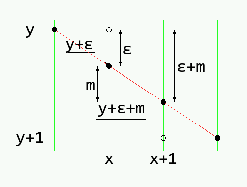
Drawing a line on a raster grid.

In this example the pixel (x, y) is activated, the next pixel to be activated lies at (x+1, y+1). The gradient is m and ε is the y-ordinate error. (The figure has been changed from the original, so that y increases down the page).

Pixel Coordinates

Most textbooks treat the pixel on the coordinate intercept, however when using an image editor the pixel is shown in the centre of a square, so point 0,0 is the middle of the square in the upper left corner.

In effect the choice lies between which of the two y values is closer, y or y+1 at the new x value of x+1.

The plotted point (x, y) is usually in error by an amount ε from the mathematically correct plot. The mathematical plot is at (x, y+ε). This error can range from -0.5 to +0.5. In moving from x to x+1 the value of the mathematical y-ordinate would be y+ε+m. Choose the next coordinate as (x+1, y) if the difference between the new value and y is less than 0.5.

\[y + \epsilon + m < y + 0.5\]

Otherwise plot (x+1, y+1). This minimises the total error between the mathematical line and what is displayed. The error resulting from this new point can now be written back into ε which allows the process to repeat for the next point at x+1. The new error can have one of two values, depending on which new point is plotted. If (x+1, y) is chosen, then the new error is given by:

\[\epsilon_{new} \leftarrow (y + \epsilon + m) - y\]

otherwise:

\[\epsilon_{new} \leftarrow (y + \epsilon + m) - (y + 1)\]

This allows us to create an algorithm based on the error.

\[\begin{split}\begin{align} & \epsilon \leftarrow 0; \, y \leftarrow y_{1} \\ & for \, x \leftarrow \, x_{1} \, to \, x_{2} \, do \\ & \quad Plot \, point \, at \, (x,y) \\ & \quad if \, ( \epsilon + m < 0.5 ) \\ & \qquad \epsilon \leftarrow \epsilon + m \\ & \quad else \\ & \qquad y \leftarrow y + 1, \, \epsilon \leftarrow \epsilon - 1 \\ & \quad endif \\ & endfor \end{align}\end{split}\]

To eliminate the floating point numbers multiply the inequality after the plot throughout by Δx then by 2.

\[\begin{split}& \epsilon + m < 0.5 \\ & \epsilon + \Delta{y}/\Delta{x} < 0.5 \\ & 2 \epsilon \Delta{x} + 2 \Delta{y} < \Delta{x}\end{split}\]

Now the comparison only uses integers.

Substitute ε' for ε Δx

\[2(\epsilon' + \Delta{y}) < \Delta{x}\]

The update rules for the error on each step may also be cast into the ε' form.

\[\begin{split}& \epsilon \leftarrow \epsilon + m \\ & \epsilon \leftarrow \epsilon + m - 1\end{split}\]

multiplying by Δx gives

\[\begin{split}& \epsilon \Delta{x} \leftarrow \epsilon \Delta{x} + \Delta{y} \\ & \epsilon \Delta{x} \leftarrow \epsilon \Delta{x} + \Delta{y} - \Delta{x}\end{split}\]

convert to ε' form

\[\begin{split}& \epsilon' \leftarrow \epsilon' + \Delta{y} \\ & \epsilon' \leftarrow \epsilon' + \Delta{y} - \Delta{x}\end{split}\]

convert the algorithm

\[\begin{split}\begin{align} & \epsilon' \leftarrow 0; y \leftarrow y_{1} \\ & for \, x \leftarrow x_{1} \, to \, x_{2} \, do \\ & \quad Plot \, point \, at \, (x,y) \\ & \quad if \, ( \, 2 (\epsilon' + \Delta{y}) < \Delta{x} ) \\ & \qquad \epsilon' \leftarrow \epsilon' + \Delta{y} \\ & \quad else \\ & \qquad y \leftarrow y + 1, \, \epsilon' \leftarrow \epsilon' - + \Delta{y}) < \Delta{x} \\ & \quad endif \\ & endfor \end{align}\end{split}\]

In order to draw lines in every situation, the algorithm is modified in such a way that the calculation continues to work normally, by changing the start and end points and changing back as necessary.

m > 1

For a steep slope exchange all the x-values for y-values, and the old y-values become x-values. After the calculation swop the values back again.

x0 > x1

If the start x-coordinate is higher than the end x-coordinates swop the start and end points.

m < 0

Change the variables so as to make a positive gradient, so (x0, y0) (x1, y1) is transformed to (x0, -y0) (x1, -y1) then after the algorithm is calculated change the sign of all y-values.

As the changes are not totally exclusive it is found that just using the first and second will cover the third case.

The first script explicitly shows the changes that are required to operate in all 8 octants (2 octants make a quadrant)

Show/Hide Bresenham First Variant

def bresenham(origin, dest, fill=(0,0,0)):
 result = []
 x0 = origin[0]; y0 = origin[1]
 x1 = dest[0]; y1 = dest[1]

 steep = abs(y1 - y0) > abs(x1 - x0)
 if steep:
     x0, y0 = y0, x0
     x1, y1 = y1, x1

 backward = x0 > x1
 if backward:
     x0, x1 = x1, x0
     y0, y1 = y1, y0

 dx = x1 - x0
 dy = abs(y1 - y0)
 error = dx / 2
 y = y0

 if y0 < y1: ystep = 1
 else: ystep = -1

 # the next few lines are the algorithm
 for x in range(x0, x1+1):
     if steep: result.append((y,x))
     else: result.append((x,y))
     error -= dy
     if error < 0:
         y += ystep
         error += dx
 # ensure the line extends from the starting point to the destination
 # and not vice-versa
 if backward: result.reverse()

 return result

The requirements for universality can easily be seen, however this script was not used.

Bitwise Operations

To speed up the multiplication use a bit left shift operation, so when there is a value multiplied by 2 convert to << 1:

D = 2*dy - dx
.....
   D -= 2*dx
D += 2*dy

becomes:

D = (dy<<1) - dx
....
   D -= dx<<1
D += dy<<1

The following script was preferred

Show/Hide Bresenham Second Variant

def bresenham(x0, y0, x1, y1):
 """Yield integer coordinates on the line from (x0, y0) to (x1, y1).
 Input coordinates should be integers.
 The result will contain both the start and the end point.
 """
 dx = x1 - x0
 dy = y1 - y0

 xsign = 1 if dx > 0 else -1
 ysign = 1 if dy > 0 else -1

 dx = abs(dx)
 dy = abs(dy)

 if dx > dy: # gentle slope
     xx, xy, yx, yy = xsign, 0, 0, ysign
 else:       # steep slope
     dx, dy = dy, dx
     xx, xy, yx, yy = 0, ysign, xsign, 0

 D = (dy<<1) - dx
 y = 0

 for x in range(dx + 1):
     yield x0 + x*xx + y*yx, y0 + x*xy + y*yy
     if D >= 0:
         y += 1
         D -= dx<<1
     D += dy<<1

Only the steep slope situation was explicitly scripted, the backward slope was incorporated into additional variables. The change of the multiplication to a bitwise function was straightforward.

Both these scripts can be changed to point plotting. In the first case wherever the script appends to a list plot a point, also the final condition for backward and reversal becomes irrelevant. With the second script the yield statement is replaced by a point plot using the given coordinates.