Antialiased Arc#
Since PIL already has a normal arc, which can be widened by using two filled pieslices, there is no real need to duplicate this. Work with the thick antialiased circle script as the basis for the antialiased arcs, as it can show the range of thicknesses we require.
One might try drawing a circle then erasing the unwanted part, quite apart from a wasteful circle plot where normally the larger part is plotted then overplotted by a figure in the background colour, the surrounding area needs to be empty, which is not always the case. Provided there is access to a circle script it can be readily transformed into an arc by turning the plotting on or off according to our needs.
Show/Hide Circles and Line 5 to 12 Radius
Antialiased Circles 5 to 12 Pixel Radius with 45° Line |
|---|

|
|
|
|
|
|
|
|
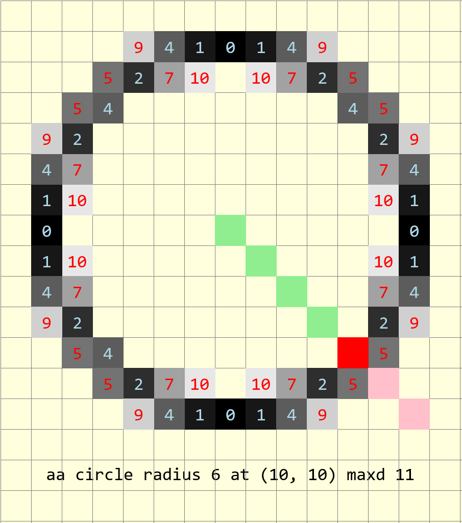
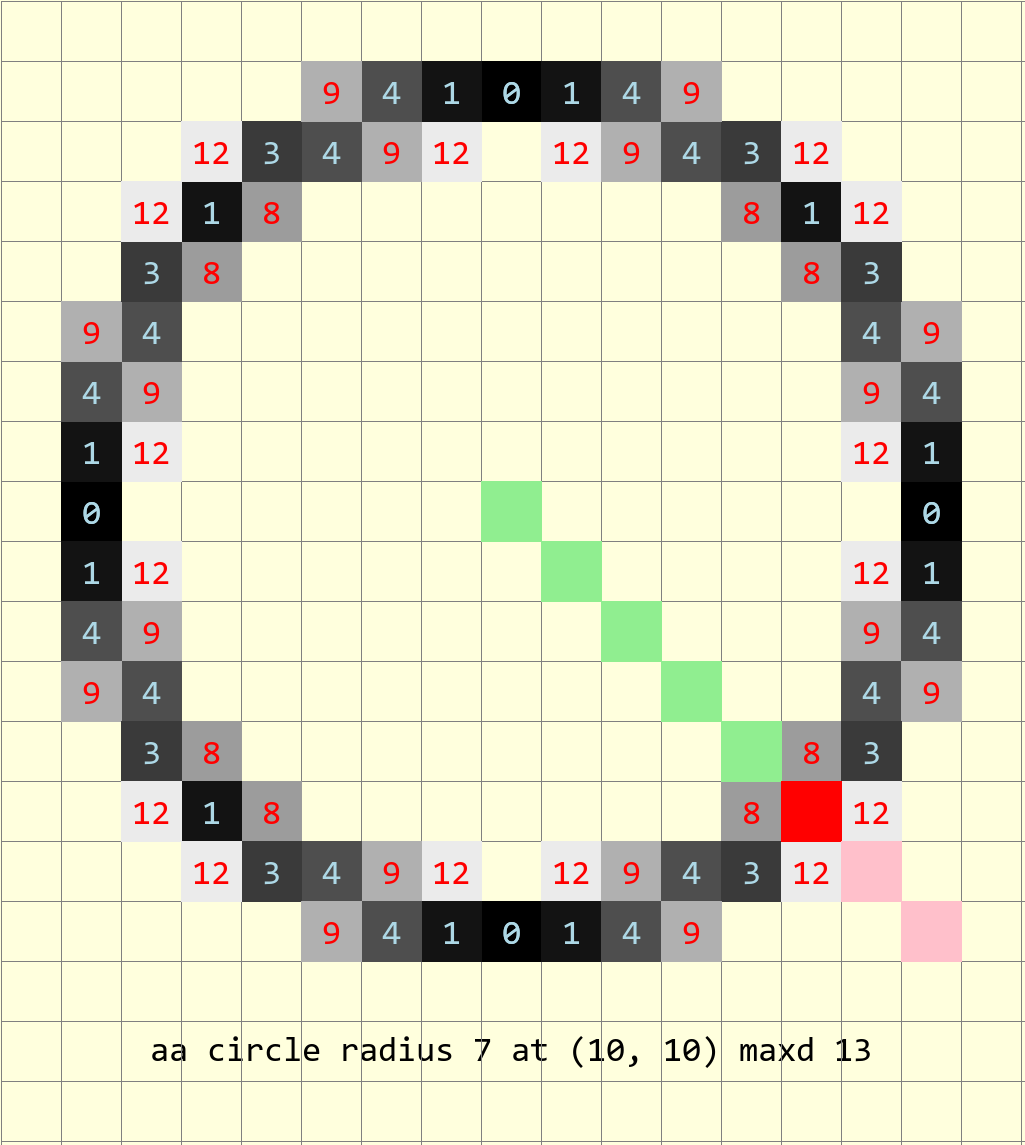
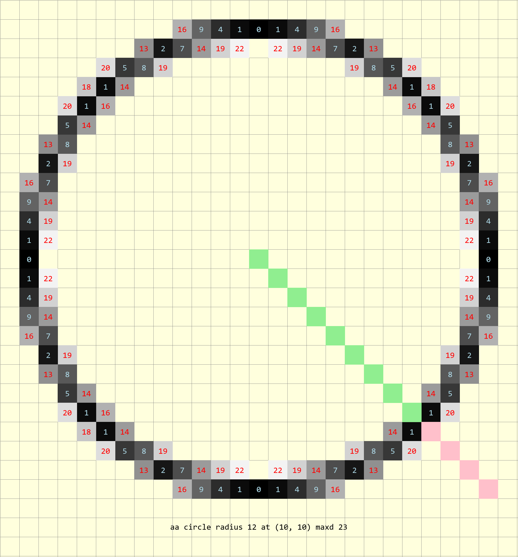
The alternative is to convert the start and finish angles to coordinates, then turn the plotting on and off in each of the octants. There is an element of uncertainty since the circle might not pass through these points. (We have already seen that the 45° angle might or might not intercept the circle on a pixel, but fall between two pixels). Drawing a 45° line, that has a colour change with length about the radius. When shorter than the radius the colour is light green, when longer than the radius the colour is pink, just on the radius the line is red. Even with the limit of ± 0.5 the radius is missed 3 times out of 8 in our sample. Where the red pixel shows, it most often is on the circle, rather than between 2 pixels on the circumference. A simple intercept is therefore doubtful, a better method is required.
If the slope of the normal is calculated then this is simple but a comparatively costly calculation compared to the Bresenham circle plot. It involves calculating the difference in y values divided by the difference in x values, where the points on the circumference are computed against the circle's centre. Since we are only computing in one sector (octant) we know that one of the two ordinates will change at every point along the circumference. When plotting around the circle we have already the seen the eight way symmetry, in each quadrant the two plots have a shallow and a steep slope (drawing a line from the circle centre to the plotted point). At each major axis the pixels are plotted from the major axis towards the 45° line, so in the first sector the plot starts at (r,0) and advances clockwise, whereas in the eighth sector it also starts from (r,0) but advances anticlockwise. When drawing a circle the fourth sector (second quadrant) is used to calculate the plot so when comparing slopes take the absolute values, then compute its steep twin in the third sector.
Plotting the start and finishing slopes up until 180° there are 4 different situations, with both start and finish in the same sector and progressing until the start and finish are separated by two full sectors. This means that we need to plot situations where both points are in the same sector, only one point is in its own sector or just plot a full sector plot.
When both plots are in the same sector plotting is turned on when it meets one of the points and turned off again when it meets the other point. If only a single plot is in a sector whether the plotting is turned on or off depends on the overall geometry and where the plotting starts relative to the point.
Start by sorting out the required conditions for both points in the same sector. Plotting will begin once the actual slope is greater than or equal to the starting slope, then switched off again if the actual slope is greater than or equal to the finishing slope. If both points are in a steep sector then use an inverse slope value to see whether the slope is less than or equal to the final slope then the starting slope. The computed value is the inverse of the actual slope, with a small addition to the y-value to prevent having an infinite slope when y is zero.
Before plotting assess which sectors the start and finishing points are located, this then determines whether the plotting is switched on from the start or not. Indicate the sector value from the arc control function to the circle plotting function. If there is only one point in a sector indicate by having 0 for the inactive point. When plotting a full sector indicate it with both sector numbers being negative. The plotpoint function has been changed to only plot if one or both sectors are activated, the negative sector values are made positive before checking which sector to plot.
A separate function is used to find the sector (octant) and quadrant.
Show/Hide Show Point Sector findQuad
def findQuad(xm, ym, x, y):

    dx = x - xm
    dy = y - ym
    gradient = abs(dy/dx)

    # check which quadrant(s) left and right lines are in
    # 1st quadrant
    if (x > xm and y >= ym):
        dX = +dy
        dY = -dx
        quad = 1
        sect = 2 if gradient > 1 else 1
    # 2nd quadrant
    if (x <= xm and y > ym):
        dX = -dx
        dY = -dy
        quad = 2
        sect = 3 if gradient > 1 else 4
    # 3rd quadrant
    if (x < xm and y <= ym):
        dX = -dy
        dY = +dx
        quad = 3
        sect = 6 if gradient > 1 else 5
    # 4th quadrant
    if (x >= xm and y < ym):
        dX = +dx
        dY = +dy
        quad = 4
        sect = 7 if gradient > 1 else 8

return quad, sect
Use a modified plotpoint function.
Show/Hide Plot Points by Sector plotpoints
def plotpoints(dr, xm, ym, x, y, sects, fill, all8=1):
    # plots all 8 sectors or only 4 sectors in the while loop
    if sects[0] < 0:
        ltemp = list(sects)
        ltemp[0] = -ltemp[0]
        sects = tuple(ltemp)

    if all8 == 1:
        if sects[0] == 1 or sects[1] == 1:
            dr.point((xm-x, ym+y), fill)               # I Octant
        elif sects[0] == 3 or sects[1] == 3:
            dr.point((xm-y, ym-x), fill)               # III. Octant
        elif sects[0] == 5 or sects[1] == 5:
            dr.point((xm+x, ym-y), fill)               # V  Octant
        elif sects[0] == 7 or sects[1] == 7:
            dr.point((ym+y, xm+x), fill)                #   VII. Octant

    if sects[0] == 4 or sects[1] == 4:
        dr.point((xm+x, ym+y), fill)               #  IV . Octant
    elif sects[0] == 2 or sects[1] == 2:
        dr.point((ym+y, xm-x), fill)               # II Octant
    elif sects[0] == 8 or sects[1] == 8:
        dr.point((xm-x, ym-y), fill)               #  VIII. Octant
    elif sects[0] == 6 or sects[1] == 6:
        dr.point((xm-y, ym+x), fill)               # VI Octant
The thick antialiased circle is modified to switch the plotting on or off,
using the variable plot. During the main while loop compute the
actual slope and its inverse, compare to the start and finish slopes, then
turn the plotting on or off. Only plot when the variable plot is 1.
Otherwise the circle plot is unchanged apart from signalling to plotponts
in which sector to plot.
Show/Hide Wide Antialiased Circle plotCircle
def plotCircle(dr, xm, ym, r, start, finish, width, sects, fill=(0,0,0),
                back=(0,0,0)):
    # xm, ym = centre
    # draw an antialiased circle on light background
    r0 = r
    x = -r
    y = 0                               # IV. Octant from left to bottom left

    err = 2 - 2 * r                         # initial difference

    sslope = abs((ym-start[1])/(xm-start[0]))
    fslope = abs((ym-finish[1])/(xm-finish[0]))
    # check sects
    ssect = 0
    fsect = 0
    plot = 0
    ssect, fsect = sects
    if sects[0] == sects[1]:
        # start, finish in one sector
        plot = 0
    elif (sects[0] == 0 and sects[1] in (1,3,5,7)) or \
        (sects[0] in (2,4,6,8) and sects[1] == 0):
        plot = 1

    if sects[0] < 0:
        plot = 1

    maxdi = [0]
    for n in range(0, width+1):
        maxdi.append(maxdi[n] + 2 * (r-n) -1)
    maxdi.remove(0)
    maxd = maxdi[0]
    # ensure inner aa working with conditions for single aa
    # find maxd of smallest main circle
    maxdsm = 2 * (r-width+1) - 1
    # thick factor used outer main lines
    thfact = (width-1)/2

    def errs(comp, size,j):
        return 255 if comp == 255 else int((255-comp) * j / size) + comp

    diffs = defaultdict(list)
    diffs = defaultdict(lambda:back, diffs)
    for i in range(maxd):
        if fill == (0,0,0):
            diffs[i] = tuple(int(255*i/maxd) for k in range(3))
        else:
            diffs[i] = tuple(errs(fill[k],maxd,i) for k in range(3))

    diffsm = defaultdict(list)
    diffsm = defaultdict(lambda:back, diffsm)
    for i in range(maxdsm):
        if fill == (0,0,0):
            diffsm[i] = tuple(int(255*i/maxdsm) for k in range(3))
        else:
            diffsm[i] = tuple(errs(fill[k],maxdsm,i) for k in range(3))

    while -x > y - 1:
        # actual slope and its inverse
        aslope = abs((-y)/(-x))
        cslope = abs(-x/(y+0.2))

        if ssect in (1,5) and plot == 0:
            if aslope >= sslope:
                plot = 1
        elif fsect in (1,5) and plot == 1:
            if aslope >= fslope:
                plot = 0
        elif fsect in (2,6) and plot == 0:
            if cslope <= fslope:
                plot = 1
        elif ssect in (2,6) and plot == 1:
            if cslope <= sslope:
                plot = 0
        elif ssect in (3,7) and plot == 0:
            if cslope <= sslope:
                plot = 1
        elif fsect in (3,7) and plot == 1:
            if cslope <= fslope:
                plot = 0
        elif fsect in (4,8) and plot == 0:
            if aslope >= fslope:
                plot = 1
        elif ssect in (4,8) and plot == 1:
            if aslope >= sslope:
                plot = 0

        err0 = err
        e2 = err-(2*y+1)-(2*x+1) # abs(err+2*(x+y)-2)
        ea = abs(e2)
        out = max(0,int(ea-thfact)) #*maxd/10)
        if plot == 1:
            plotpoints(dr, xm, ym, x, y, sects, (diffs[out] if out > 0 else fill),
                all8 = (1 if (xm+x, ym+y) != (xm-y, ym-x) \
                or (x==-r and y == 0) else 0))

        # fill out diagonals
        x0 = -x
        eout = abs(e2 + 2*x0 + 2*y + 2)
        if eout < maxd: # and (width-1)//2 == 0
            if plot == 1:
                plotpoints(dr, xm, ym, x-1, y+1, sects, (diffs[eout] if eout > 0 else fill),
                    all8 = (1 if (xm+x, ym+y) != (xm-y, ym-x) else 0))

        ein = e2
        x0 = -x
        for n in range(0, width):
            ein = ein-(2*(x0-n)-1)
            e0 = -ein

            if n < width-2:
                fact = fill
            elif n == width-1:
                fact = diffs[abs(int(e0-maxd*thfact/10))] if n==0 else \
                    diffsm[e0-maxdi[n-1]]
            else:
                fact = diffsm[max(0,int(abs(e0-maxdi[n])-maxdsm*thfact/10))]
            if plot == 1:
                plotpoints(dr, xm, ym, x+n+1, y, sects, fact,
                    all8 = (1 if (xm+x, ym+y) != (xm-y, ym-x) else 0))

        if (err0 <= y):
            y += 1
            err += y * 2 + 1            # e_xy+e_y < 0

        if (err0 > x or err > y):          # e_xy+e_x > 0 or no 2nd y-step
            x += 1
            # aa missed by diagonals
            eout = abs(e2 + 2*y - 1)
            if eout < maxd:
                if plot == 1:
                    plotpoints(dr, xm, ym, x-1, y, sects, (diffs[eout] if eout > 0 else fill),
                        all8 = (1 if (xm+x, ym+y) != (xm-y, ym-x) else 0))
            err += x * 2 + 1            # -> x-step now
The user interracts with the arc control
function make_arc, which handles the overall geometry of the arc, and
controls how many passes over the circle plot are required.
Show/Hide Arc Control make_arc
def make_arc(dr, xm, ym, r, start, finish, width, fill=(0,0,0), back = (255,255,221)):

    sq = findQuad(xm, ym, start[0], start[1])
    fq = findQuad(xm, ym, finish[0], finish[1])
    sects = ()

    diff_sect = fq[1] - sq[1]

    if diff_sect == 0:          # both end points in same sector
        sects = sq[1],fq[1]
        plotCircle(drawl, xm, ym, r, start, finish, width, sects,
            fill=(0,0,0), back = (255,255,221))

    elif (diff_sect == 1) or (sq[1] == 8 and fq[1] == 1):
        sects = sq[1],0
        plotCircle(drawl, xm, ym, r, start, finish, width, sects,
            fill=(0,0,0), back = (255,255,221))

        sects = 0,fq[1]
        plotCircle(drawl, xm, ym, r, start, finish, width, sects,
            fill=(0,0,0), back = (255,255,221))

    elif (diff_sect == 2) or (sq[1] == 8 and fq[1] == 2) or (sq[1] == 7 and fq[1] == 1):
        sects = sq[1],0
        plotCircle(drawl, xm, ym, r, start, finish, width, sects,
            fill=(0,0,0), back = (255,255,221))
        if sq[1] < 8:
            sects = -sq[1]-1,-sq[1]-1
        else:
            sects = -1,-1
        plotCircle(drawl, xm, ym, r, start, finish, width, sects,
            fill=(0,0,0), back = (255,255,221))
        sects = 0,fq[1]
        plotCircle(drawl, xm, ym, r, start, finish, width, sects,
            fill=(0,0,0), back = (255,255,221))

    elif (diff_sect == 3) or (sq[1] == 8 and fq[1] == 3) or (sq[1] == 7 and fq[1] == 2):
        sects = sq[1],0
        plotCircle(drawl, xm, ym, r, start, finish, width, sects,
            fill=(0,0,0), back = (255,255,221))

        if sq[1] < 7:
            sects = -sq[1]-2,-sq[1]-2
        else:
            sects = -1,-1
        plotCircle(drawl, xm, ym, r, start, finish, width, sects,
            fill=(0,0,0), back = (255,255,221))

        if sq[1] < 8:
            sects = -sq[1]-1,-sq[1]-1
        else:
            sects = -2,-2
        plotCircle(drawl, xm, ym, r, start, finish, width, sects,
            fill=(0,0,0), back = (255,255,221))

        sects = 0,fq[1]
        plotCircle(drawl, xm, ym, r, start, finish, width, sects,
            fill=(0,0,0), back = (255,255,221))
It can be seen that once the initial conditions are made for both start and finishing points that the other situations are met when there is only a single point in a sector.
Although an arc normally requires a start and finish angle, the situation often occurs that two enclosing lines already exist. This means that the lines' slopes are easily computed, which allows us to avoid a trignometric calculation. One can easily add an angle to the make_arc function and change it to coordinates.